Line Balancing

Some Background

Like my other posts, the inspiration for this came from a class I recently took on optimization. While the course mostly covered linear and mixed integer programming, there were hosts of examples covering many use cases. Oddly enough, I have been thinking about writing a script to automate line balancing for a while now but lacked the inspiration to just sit down and do it. I have looked for solutions using solvers in the past, but most end up being schedulers that lack a focus on maximizing utilization or just require way too much manual hard coding. The book we were using had a good example of a typical line balance problem, so I thought I would port it over to Python and make some minor tweaks to generalize the application. I think I have made a program that is about 95% automated, save for entering cycle times and the sequence of process steps. Put in your own process and give it a test drive.

tl;dr Run the script in the cloud here: Colab Notebook

What is a Line & Why Should it be Balanced?

Line Balancing is one of the simplest, yet most impactful tools that an Industrial Engineer has in their toolkit. When we talk about a line, we are talking about an assembly line, or a series of workstations that work in sequence. In a manufacturing environment, line balancing is the science of distributing process steps across a set of workstations to minimize the number of workstations, \(W\), and maximize utilization, \(u\), while still meeting the takt time. This minimizes WIP and through balancing of cycle times at each station, maximizes utilization, reducing waiting time. Because line balancing, in its simplest form, takes the process as-is, and simply rearranges the tasks, it can provide an incredible return on investment for unbalanced systems.

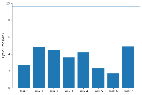
Line balancing is all about maximizing output to the takt time, but why is this important? When we think about a production line, it is like an accordion. We know from Little’s Law that at steady state, a system outputs at the bottleneck rate, \(r_b\). In its fastest, but likely least balanced form, each distinct process step has its own workstation. This leads to the most workstations, but the lowest \(r_b\). In The process below, the system will produce a part every 4.9 minutes at the last station. However, you notice that there is quite some space between the top of each bar and the takt time of 9.6. This is where utilization is important. To minimize costs, we want to create product at the speed we consume it, or the taxt time. No more, no less. If the takt time is below \(r_b\), we can look at combining steps to reduce the number of workstations and increase utilization. As takt decreases towards \(r_b\), we can continue to add process steps, unfolding the line with more stations, to lower the \(r_b\) of the system and still meet the takt.

While performing line balancing seems simple, this quickly gets complicated as process dependencies emerge and meaningful reductions in cycle times may require significant re-engineering of the product or process. It is not always as simple as adding more labor or stations to the system. After all, to minimize WIP, we want to minimize the number of stations \(W\), and to reduce costs, we want to maximize line utilization. With this simple objective and constraints, an optimization problem is born.

But First, A Disclaimer

We can manually balance a line with good old-fashioned whiteboards and post-it notes. Frankly, it is probably quicker in most cases. However, this blog isn’t about applying pragmatic solutions to complex problems—we like to indulge ourselves in automation and high-tech tools for even the simplest use cases. For today’s exercise in self-indulgence, we are exploring the application of Mixed Integer Programming (MIP) to automate our line balancing problems.

MIP & The Line Balancing Problem

Now, there are a couple options for solving MIP problems, and optimization in general. There’s PuLP, CPLEX, Gurobi, and many more free and costly options. Today, we’ll be using Google’s OR-Tools.

Now you may ask, why MIP and not a regular LP? The Line Balancing Problem is a type of assignment problem, where binary variables are assigned. In our case, \(X_{ij}\) is 1 if station \(i\) is assigned process \(j\).

In our use case, the process is happening at that station, or not, and it cannot be anything in between. As we add constraints to the system, in a very simple case, this can produce an optimized result with a linear solver that isn’t actually workable in reality. For example, it may suggest we have 3.26 stations, when we can only have 3 or 4, but not in between. This may seem simpler, but is computationally more complicated, and requires us to use a MIP solver.

Problem Overview

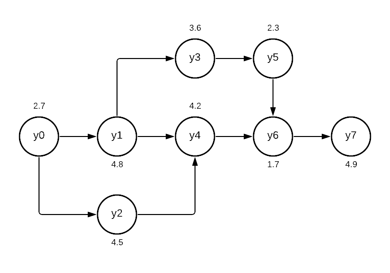
Let us imagine an eight-step process to build a widget that we are balancing. Besides this, our factory is available for eight hours a day, and we have a demand of 50 widgets per day. Times below are in minutes.

Note: You’re probably wondering why I labeled the process steps \(y_0, y_1, \dots, y_7\). This was to align with the zero-based array indexing in Python. This way, y[0] \(= y_0\) and not \(y_1\). You will notice this convention carries into the variable names in our mixed integer program. I found it easier to wrap my mind around when converting between array indexes and the actual variable I was looking for.

Before we enter the data into our program, let us pull in the packages and initialize our solver. We are going to use SCIP, but there are other options.

from ortools.linear_solver import pywraplp
import numpy as np
import pandas as pd
import matplotlib.pyplot as plt

solver = pywraplp.Solver.CreateSolver('SCIP')

Based on the process flow, we can enter our data in an calculate our current line utilization.

no = 8  # number of process steps
steps = list(range(0, no))
process = ['Task %s' % s for s in steps]

ct = [ # cycle times
    2.7, # y0
    4.8, # y1
    4.5, # y2
    3.6, # y3
    4.2, # y4
    2.3, # y5
    1.7, # y6
    4.9, # y7
]

seq = np.array([ # predecessor , task
    [0,1], # y0 is before y1....
    [0,2],
    [1,3],
    [1,4],
    [2,4],
    [3,5],
    [4,6],
    [5,6],
    [6,7],
])

avail = 8 * 60  # 8 hours converted to minutes
demand = 50
takt = avail / demand
util = sum(ct) / (takt * len(process))
rb = max(ct)

print ('Utilization:', util)
print ('Takt:', takt)
print ('r_b:', rb)

Utilization: 0.37369791666666674
Takt: 9.6
r_b: 4.9

Alright, not so great. With the system \(r_b = 4.9\) and the \(\text{Takt}=9.6\), we can see why the utilization is so low. To visualize this, we can put the data into a bar plot with the takt time.

fig = plt.figure()
ax = fig.add_axes([0,0,1,1])
ax.set_ylabel('Cycle Time (Min)')
ax.bar(process,ct)
ax.axhline(y=takt)
plt.show()

We would like to have our cycle time at each station closer to the takt time to increase utilization. This will ensure that widgets exit the system at a rate equal to or faster than the demand, ensuring we keep our customers happy. A \(r_b > \text{Takt}\) doesn’t make enough parts in the day (too slow), and a \(r_b < \text{Takt}\) produces parts at a rate faster than we need them. Ideally \(r_b = \text{Takt}\), but we try to shoot for a little below to be safe.

Defining Constraints

We have talked about minimizing a couple things now, specifically utilization through \(W\). To use a MIP solver, we need to translate our line balancing issue into and equation that can be minimized. To start, we need to initialize a decision variable for each task so we can assign a sequence.

infinity = solver.infinity()
y = {}

# create a integer variable yi for each process step
for i in range(len(process)):
    y[i] = solver.IntVar(0, infinity, 'y%i' % i)

Following this, we need to create a binary variable for each \(X_{ij}\) where \(X_{ij}= 1\) if station \(i\) is assigned process \(j\). We have eight process steps that can be performed at eight stations, resulting in 64 variables.

a = 0
x= {}

for i in range(len(process)):
    for j in range(len(process)):
        x[a] = solver.IntVar(0, 1, 'x%i%i' % (i, j))
        a += 1

Next up, we want to put in the sequence of tasks as a constraint. Since we are using integers, we can assign each unique process step a sequential value to ensure that we do not get things out of order. By using the sum of these values, we can create a simple way to ensure tasks do not get assigned to stations in the wrong order. For example, we can make sure Task 1 is before Task 2 with the constraint below. We will reference the sequence using our seq array.

for i in range(len(seq)): # sequence constraints
    solver.Add(y[seq[i,0]] - y[seq[i,1]] <= 0)

If \(Y_0\) is assigned \(X_{0j}\) tasks where \(X_{0j} > X_{1j}\), it will cause \(Y_0 > Y_1\), breaking the constraint. We will add in another constraint that increments the value of \(Y_i\) based on the step it was assigned so this piece works.

for i in range(len(process)): # set Yi to enforce sequencing
    constraint_expr = \
    [(j+1) * x[((i*7)+j+(i*1))] for j in range(len(process))]
    solver.Add(sum(constraint_expr) == y[i])

We want to make sure each station does not have more than the takt time worth of work at the station. The equation is the sum of each task \(j\) iterated across station \(i\) must be \(\leq \text{Takt}\). We also want to set the correct cycle time from our ct array as the coefficient for its respective \(X_{ij}\) variable.

for i in range(len(process)): # station CT does not exceed takt
    constraint_expr = \
    [ct[j] * x[i+(j*8)] for j in range(len(process))]
    solver.Add(sum(constraint_expr) <= takt)

Another requirement is that we only performed each process at one station. We express this as

for i in range(len(process)): # a given task is only at one station
    constraint_expr = \
    [x[((i*7)+j+(i*1))] for j in range(len(process))]
    solver.Add(sum(constraint_expr) == 1)

Last, we want to pull the whole program together with our global variable to minimize \(Z\). In the same way we incremented the \(Y_i\) with process steps, we will create a constraint that increments \(Z\) every time a station is “activated” with a task. Since our aim is to minimize the number of stations, our objective function is quite simple:

To initialize this variable, we need to create a new integer with z = solver.IntVar(0, infinity, 'z').

In the previous step, we talked about creating a constraint that links the activation of \(Y_i\) to \(Z\). This is achieved rather simply.

for i in range(len(process)):
    solver.Add(y[i] <= z)

The Mixed Integer Program

We have reached the end, and we can reflect so far on what we’ve accomplished. Outside of the specific sequence constraints (the \(Y_i - Y_{i+x} \leq 0\) stuff), the rest of the constraints should apply to almost any assembly line, and scale with size. Do not let the summation notation scare you, it’s mostly a bunch of monotonous addition. Below is our mixed integer program in all its glory.

Using the Solver

We are ready to optimize. This is as simple as executing solver.Minimize(z), but requires a little more code to get anything meaninful.

status = solver.Solve()
if status == pywraplp.Solver.OPTIMAL:
    print('Number of Stations =', solver.Objective().Value())
else:
    print('The problem does not have an optimal solution.')

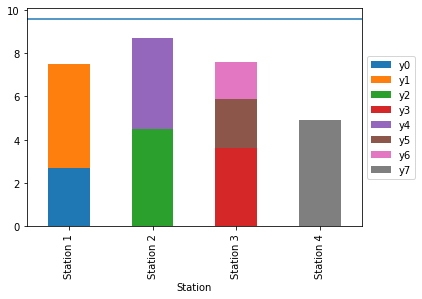
Number of Stations = 4.0

The results are out, and we know we can run this process with four stations, which is half of what we previously had. Now, let us visualize what the new process looks like.

station = []
task = []
names = ['Station %s' % s for s in station]

for j in range(len(process)):
    station = np.append(station, ['Station %s'
                        % int(y[j].solution_value())], axis=0)
    task = np.append(task, [y[j].name()], axis=0)

line = pd.DataFrame({'Task': task, 'CT': ct, 'Station': station})

ax = line.pivot('Station', 'Task', 'CT').plot(kind='bar', stacked=True)
ax.axhline(y=takt)
ax.legend(loc='center left', bbox_to_anchor=(1, 0.5))
plt.show()

util = sum(ct) / (takt * solver.Objective().Value())
print ('Utilization:', util)

Outstanding, now we can see the new sequence of process steps and layout of the line. Our utilization is up to almost 75%, almost double from our baseline and right where we want the system running at.

I hope you found this tutorial educational, and I hope you can use the code to automate your next line balancing activity. Outside of inputting cycle time and sequence, be able to simply add or subtract process steps and the rest of the program should work automatically. Let me know if you have a success story!

Acknowledgements

The framework and approach for this post was adapted from Radsdale’s (2014) Spreadsheet modeling and decision analysis for Python with Google’s OR-Tools. Reference below.

Ragsdale, Cliff. Spreadsheet modeling and decision analysis: a practical introduction to business analytics. Cengage Learning, 2014.

Full Program

If you do not have a Python IDE, you can run this in the cloud! Check out my Colab Notebook. Remember you have to restart the runtime after executing the first cell. This simply means clicking the Play button again once it prompts to restart the runtime. Happy line balancing!

from ortools.linear_solver import pywraplp
import numpy as np
import pandas as pd
import matplotlib.pyplot as plt

solver = pywraplp.Solver.CreateSolver('SCIP')

no = 8  # number of process steps
steps = list(range(0, no))
process = ['Task %s' % s for s in steps]

ct = [ # cycle times
    2.7, # y0
    4.8, # y1
    4.5, # y2
    3.6, # y3
    4.2, # y4
    2.3, # y5
    1.7, # y6
    4.9, # y7
]

seq = np.array([ # predecessor , task
    [0,1], # y0 is before y1....
    [0,2],
    [1,3],
    [1,4],
    [2,4],
    [3,5],
    [4,6],
    [5,6],
    [6,7],
])

avail = 8 * 60  # 8 hours converted to minutes
demand = 50
takt = avail / demand
util = sum(ct) / (takt * len(process))
rb = max(ct)

print ('Utilization:', util)
print ('Takt:', takt)
print ('r_b:', rb)

fig = plt.figure()
ax = fig.add_axes([0,0,1,1])
ax.set_ylabel('Cycle Time (Min)')
ax.bar(process,ct)
ax.axhline(y=takt)
plt.show()

infinity = solver.infinity()
y = {}

# create a integer variable yi for each process step
for i in range(len(process)):
    y[i] = solver.IntVar(0, infinity, 'y%i' % i)

a = 0
x= {}

for i in range(len(process)):
    for j in range(len(process)):
        x[a] = solver.IntVar(0, 1, 'x%i%i' % (i, j))
        a += 1

for i in range(len(seq)): # sequence constraints
    solver.Add(y[seq[i,0]] - y[seq[i,1]] <= 0)

for i in range(len(process)): # set Yi to enforce sequencing
    constraint_expr =     [(j+1) * x[((i*7)+j+(i*1))] for j in range(len(process))]
    solver.Add(sum(constraint_expr) == y[i])

for i in range(len(process)): # station CT does not exceed takt
    constraint_expr =     [ct[j] * x[i+(j*8)] for j in range(len(process))]
    solver.Add(sum(constraint_expr) <= takt)

for i in range(len(process)): # a given task is only at one station
    constraint_expr =     [x[((i*7)+j+(i*1))] for j in range(len(process))]
    solver.Add(sum(constraint_expr) == 1)

z = solver.IntVar(0, infinity, 'z')

for i in range(len(process)):
    solver.Add(y[i] <= z)

solver.Minimize(z)

status = solver.Solve()
if status == pywraplp.Solver.OPTIMAL:
    print('Number of Stations =', solver.Objective().Value())
else:
    print('The problem does not have an optimal solution.')

station = []
task = []
names = ['Station %s' % s for s in station]

for j in range(len(process)):
    station = np.append(station, ['Station %s'
                        % int(y[j].solution_value())], axis=0)
    task = np.append(task, [y[j].name()], axis=0)

line = pd.DataFrame({'Task': task, 'CT': ct, 'Station': station})

ax = line.pivot('Station', 'Task', 'CT').plot(kind='bar', stacked=True)
ax.axhline(y=takt)
ax.legend(loc='center left', bbox_to_anchor=(1, 0.5))
plt.show()

util = sum(ct) / (takt * solver.Objective().Value())
print ('Utilization:', util)

PERT, Beta, & Three-Point Approximation

I recently took a Project Management Professional (PMP) course that covered cost and schedule estimation. According to Project Management Insitute’s (PMI) Project Management Body of Knowledge (PMBOK), statistically-based estimate methods can be either parametric estimation or three-point estimate¹.

Parametric estimation, as you may have guessed, involves using the normal distribution. However, the methodology in PMBOK is not so scientific. Parametric estimation in their case is simply using linear estimation to predict a future cost. An example of this would be if Project X used \(10\) widgets at a cost of \(10\) each, and our project uses \(20\) widgets, we estimate the cost to be \(20\). Not so scientific, but certainly appropriate in certain situations.

What piqued my interest was the alternative methodology, known as a three-point estimate. The three-point estimate can be broken into two categories, one using the triangular distribution, with the other using the beta distribution (PERT method).

For the PERT methodology, the text suggests estimating parameters to produce a beta distribution which can be approximated by the normal distribution. In effect, you estimate a mean and standard deviation from your optimistic, most likely, and pessimistic estimates and use z scores to draw a tolerance interval. By its very definition (and every example they gave in the course), the three-points would produce an asymmetric distribution—otherwise, why not just estimate with a mean and standard deviation?

What wasn’t clear to me was how to bridge the gap between using parametric estimators to characterize asymmetric distributions. After some research, I ran into a book², and a corresponding website³ that explained how the PERT distribution is derived.

As it turns out, the PERT methodology uses a beta distribution function to smooth out this three-point estimate into a normal-ish distribution or a lognormal distribution². It does this by taking the three parameters and converting them into \(a_1\) and \(a_2\), the shape parameters used to create the beta smoothing.

The relationship between the two distributions can be defined as³

Where \(a\) is the optimistic estimate, \(b\) is the most likely estimate, and \(c\) is the pessimistic estimate.

Note: \(\lambda\) is usually \(4\), but from my research seems arbitrarily chosen and serves the sole purpose of weighing the most likely estimate higher than the other two.

So lets plug in some numbers here and start modeling this in R. For our model, lets say we have an activity that we estimate to cost \(a=200\), \(b=600\), \(c=1500\).

set.seed(1234)
a = 200 # optimistic
b = 600 # most likely
c = 1500 # pessimistic
lambda = 4 # arbitrary

To convert the parameters we have into a beta-smoothed PERT distribution, we need to define our shape parameters and generate some values. This can be achieved by calculating the shape parameters per Vose’s methodology³ and then scaling each sample by the range and offsetting by the optimistic estimate (see footnote link for their R code)². We need to generate at least \(10000\) samples to get a good idea of the shape of the distribution. I also took the liberty of rounding to two decimal places to make everything a bit more readable.

pert <- function(a, b, c, lambda) {
  mu = (a + lambda * b + c) / (lambda + 2)
  a1 = ((mu - a) * (2 * b - a - c)) / ((b - mu) * (c - a))
  a2 = (a1 * (c - mu)) / (mu - a)
  data = rbeta(10000, a1, a2)
  return(round(data * (c - a) + a, digits = 2))
}

If you run the function and get the quantiles (I chose \(.05, .50, .95\)) you get 5% 323.94 50% 663.6 95% 1100.46.

To get the triangular distribution with our parameters, you can simply use the rtri function from EnvStats⁴.

library(EnvStats)
tridf <- round(rtri(n = 10000, a, c, b), digits = 2)
quantile(tridf, c(.05, .50, .95)) 

We get the following quantiles 5% 361.325 50% 735.87 95% 1259.053.

Using the PMI methodology, we are given the following formulas¹:

PMI proposes using z scores to determine where 95% of the values would lie given a normal distribution, using the mean calculated and standard deviation defined above. To keep things simple, we will use the same quantile methodology as before.

mean = (a + (4 * b) + c) / 6
sd = ((c - a) / 6)
pmi <- round(rnorm(10000, mean, sd), digits = 2)
quantile(pmi, c(.05, .50, .95))  

This gets us quantiles of 5% 331.7395 50% 684.34 95% 1035.309, as well as a nice parametric distribution.

To sum it up, we have the following results:

So which method is the most accurate? That’s hard to say. I was surprised the PMI methodology got similar results to the PERT beta smoothed methodology, but I guess that is central limit theorem in action. All methods ranked probability of the extremes very low, but all three methodologies showed their bias towards the most likely scenario. Given that expert input would place some probability at both the optimistic and pessimistic, it would be interesting to compare the modeled probability with that of the expert. I would imagine its probably not \(.001\) (see this chart on how people interpret probabilistic words). Given the results, I would probably recommend padding the expert estimates to capture them within the model to the probabilistic interval they would attribute them to.

Having said that, all of this is subject to the quality of the estimates, which probably contains enough margin or error that the nuance in the equations is negligible. There is some guidance on the use of these formulas. Vose points to some research from Stanton & Farnum that to use the PMI standard deviation methodology, then the mode cannot lie more than 13% of the range from the distance to the optimistic or pessimistic value⁵. Thus, highly skewed estimates are subject to increased error in estimation.

In conclusion, I was surprised by the results here—the math seems to work out in the end, contingent on the accuracy of the estimates. The only area of improvement is possibly developing a function to pad the upper and lower estimates to get them at a probability in the model that is more aligned with the expert’s intent. Until then, happy project management activity forecasting!

Little's Law

Every factory I’ve ever worked at or been to has had one thing in common: the perception that there wasn’t enough space. I say perception because this is really more of a perspective than a statement of fact. The average workstation is generally cluttered with all sorts of things that aren’t needed for the process. A fix for this is generally 5S (which I would recommend as a great first pass), but the engineers among us will desire a more scientific approach to de-cluttering the workstation.

The answer to this is a little-known (no pun intended) theorem called Little’s Law. This theorem, thought-up by John Little, originally modeled the long-term average number \(L\) of customers in a stationary system, stating it is equal to the long-term average effective arrival rate \(\lambda\) multiplied by the average time \(W\) that a customer spends in the system. This can be expressed as ¹:

Little’s Law is also a general term for any sort of formula or theorem taking on the form \(Y=XZ\). Since we aren’t looking at queuing theory, Little’s Law in the manufacturing context is where \(\text{WIP}\) is work in process, \(\text{TH}\) is throughput, and \(\text{CT}\) is the average cycle time. Some quick thought experiments can validate this theory. Holding \(\text{TH}\) constant, if \(\text{CT}\) increases, we expect \(\text{WIP}\) to increase as well. Leveraging this, we can begin to model ideal scenarios given actual process information. In today’s post, we will focus on the relationship between \(\text{TH}\) and \(\text{WIP}\), although \(\text{CT}\) can be modeled in the same fashion².

I’ll start off with the Python code and then we can move into R. It takes about the same amount of code with either, so choose the language you are most comfortable in.

import pandas as pd
import numpy as np
import matplotlib
import matplotlib.pyplot as plt

Now, let’s generate a random process. In this case, we want 6 steps, each with a random process time of between 1-100 seconds. Alternatively, you can comment out the random chunk of code and put in your own times.

np.random.seed(1234) # set seed
process = np.random.randint(101, size=(1, 6))
# process = [18,59,30,21,78,10] 

Upon execution, our random process gives us array([[47, 83, 38, 53, 76, 24]]). Now we need to define some variables. Before we start, we have four that are part of the formulae and one that will be used to figure out a range of WIP levels to use. More details can be found about the following formulas in Factory Physics². The first variable is \(T_0\), which is the raw cycle time for the entire process. Next is \(r_b\), which is the bottleneck rate, or the slowest process divided by \(T_0\). Next is our critical WIP level, \(W_0\). This is the WIP level at which a line, with no variability in process times, that achieves maximum throughput \(r_b\) with minimum cycle time \(T_0\). The formula is \(W_0=r_bT_0\). Then we have our worst-case throughput, or \(TH_w\). This is a constant and is defined as \(\frac{1}{T_0}\). The last variable is the max range of WIP we want to model. Because our \(TH_{pwc}\) never converges with \(TH_b\), we will go with 25 times \(W_0\), which will give us room to fit most real-life scenarios and context for the full chart.

# define variables
T0 = np.amax(process)
rb = np.amax(process)/np.sum(process)
w0 = rb*T0
THw = 1/T0
maxw = int(w0*25)

After setting up our variables, we can initialize our arrays. We will want to draw three different lines in a single chart to model \(\text{TH}\) in three different ways: best case (full bottleneck speed), worst case \(1/T_0\), and the practical worse case, which gives us a threshold that should generalize to reality where the line between good and bad is.

# setup arrays for each line in the plot
wip =[] # WIP levels
THpwc =[] # practical worst case throughput
THw =[] # worst case throughput
THb = [] # best case throughput

The last step before the results is to iteratively calculate the throughput values. Python and R (or any other language for that matter) can handle this task much more elegantly than say, Microsoft Excel because we can store our results as arrays and simply graph them in a single chart. With this step, we introduce three new formulas².

# loop through our formulas and fill the arrays
for i in range(1,maxw):
    wip = np.append(wip, [i], axis=0)
    pwc = i/(w0+i-1)*rb
    THpwc = np.append(THpwc, [pwc], axis=0)
    worst = 1/T0
    THw = np.append(THw, [worst], axis=0)
    if i<w0:
        best = i/T0
    else:
        best = rb
    THb = np.append(THb, [best], axis=0)

This final step will fill our arrays so we can build our chart.

# plot our results
plt.plot(wip, THpwc, marker='', color='blue', linewidth=2, label="TH PWC")
plt.plot(wip, THw, marker='', color='red', linewidth=2, label="TH Worst")
plt.plot(wip, THb, marker='', color='green', linewidth=2, linestyle='dashed', label="TH Best")
plt.legend()
plt.show()

And there we have it. Above the blue curve is the good scenario, where below is bad. Obviously, you want to minimize WIP levels, but this chart can be used to determine a threshold for where “good enough” is. I have plotted the actual WIP level on the chart and highlighted the “good” region in the past to easily show technicians and managers an assessment of the target and future state. Use this chart to figure out ideal WIP levels and de-clutter your workstations.

For Jupyter notebooks as well as raw code for both python and R solutions, visit my repository.

For the R code, see below:

set.seed(1234)
process <- sample(1:100, 6, replace=T) # generate random process with 6 steps with times between 1-100 units time
# process <- c(18,59,30,21,78,10) # <- alternatively fill in your own process times

# define variables
T0 = max(process)
rb = max(process)/sum(process)
w0 = ceiling(rb*T0) # round to the nearest whole number
THw = 1/T0
maxw = w0*25

# setup arrays for each line in the plot
wip <- vector() # WIP levels
THpwc <- vector() # practical worst case throughput
THw <- vector() # worst case throughput
THb <- vector() # best case throughput

# loop through our formulas and fill the arrays
for (i in 1:maxw){
    wip[i] <- i
    pwc <- i/(w0+i-1)*rb
    THpwc[i] <- pwc
    worst <- 1/T0
    THw[i] <- worst
    if (i<w0){
        best = i/T0
    } else {
        best = rb
    }
    THb[i] <- best
}

# Plot the chart.
plot(wip, THw, col="red", lty=3, ylim = c(min(THw)/2,max(THb)*1.1))
lines(wip, THpwc, col="blue",lty=2)
lines(wip, THb, col="green", lty=3)

Welcome!

This is the new home for all of my posts about all things math, lean, six sigma, and statistics. I’ll be updating content on this site as I have time and come across interesting ideas.

Acknowledgments

This site is built on Jekyll is a static site generator, an open-source tool for creating simple yet powerful websites of all shapes and sizes. Find out more by visiting the project on GitHub.

The theme used on this site is called Hyde.

• Built for Jekyll
• Developed on GitHub and hosted for free on GitHub Pages
• Coded with Sublime Text 2, an amazing code editor